---
title: "A Glimpse into Quarto"
subtitle: "Reproducible & Unified Geospatial Research with Quarto"
author: "Yonghun Suh"
date: "Mar. 9, 2026"
categories: [Code]
image: https://rstudio.github.io/cheatsheets/html/images/quarto-illustration.png
format:
html:
toc: true
number_sections: true
code-copy: true
code-fold: show
code-tools: true
code-overflow: scroll
code-link: true
number-sections: true
toc_depth: 3
lightbox: true
execute:
warning: false
message: false
# freeze: true
#comments: false
---
# Introduction
## The Standard for Next-Generation Geographic Data Science: What is Quarto?
- **The Evolution of R Markdown:** R Markdown has expanded into a broader ecosystem. Developed by Posit, this system goes beyond R to encompass all aspects of scientific publishing.
- **Integration of Tools:** It allows you to freely use essential geographic research languages like R (`sf`, `terra`) and Python (`GeoPandas`) within a single document, or simply stick to the language you are most comfortable with.
- **An All-in-One Solution for Geographers:** You can complete the entire process—from data collection and spatial analysis to map visualization and final manuscript submission—within a single `.qmd` file.
## Implementing Reproducible Geography
- **Unifying Analysis and Writing:** The era of exporting maps from GIS software and pasting them into Word is over. If the underlying data changes, all maps and tables in the report are synchronized and updated in real time.
- **Reproducible & Transparent Research:** Because all code (from preprocessing to final modeling)is included in the document, fellow geographers can accurately verify and reproduce your research process.
## An Investment for the Future: Multi-Language Support and Collaboration
- **Breaking Language Barriers:** You might be using R right now, but even if you transition to Python-based spatial models later, the Quarto syntax remains exactly the same.
- [**Flawless Equation Rendering:**](#latex-math-mode) Equations essential for spatial statistics are rendered at a journal-quality level. Below is the formula for Moran's I, which measures spatial autocorrelation.
$$I = \frac{n}{\sum_{i=1}^{n}\sum_{j=1}^{n}w_{ij}} \frac{\sum_{i=1}^{n}\sum_{j=1}^{n}w_{ij}(z_i-\bar{z})(z_j-\bar{z})}{\sum_{i=1}^{n}(z_i-\bar{z})^2}$$
- **The Geographer's Portfolio:** By linking with GitHub Pages, you can publish your own research blog or project page to the world with just a few clicks.
## `One-Source, Multi-Format`: Diverse Outputs from a Single Source
- **From Reports to Papers:** After freely conducting your analysis and drafting in HTML, changing just one line in the settings converts the document into a **PDF manuscript** formatted for journal submission or an **MS Word** document for collaboration.
- **Automated Presentations:** There is no need to create a separate PowerPoint file. You can use your existing code to generate web-based slides (Revealjs). At a geography conference, simply open your browser and you are ready to present.
::: callout-tip
[Try changing `format: html` at the top of this document to `format: docx` or `format: pdf`](#sec-output-options), and then click Render again. The exact same code will instantly be converted into a Word document or a PDF paper.
:::
::: {.callout-important}
## PDF Rendering Requirement: TinyTeX
To generate **PDF** documents, Quarto requires a LaTeX distribution. I strongly recommend installing **TinyTeX**, a lightweight and portable LaTeX distribution that works seamlessly with Quarto.
You can install it by running the following command in your terminal:
```bash
quarto install tinytex
```
:::
## Why Start with HTML? (A Geographical Perspective)
- **The Magic of Interactive Maps:** Provide an experience that paper maps cannot offer. You can embed maps directly into your report, allowing readers to toggle layers on and off, or click on features to view attribute information.
- **Zero Entry Barrier:** There is no need to struggle with complex LaTeX installations. Simply click the `Render` button in RStudio, and a beautifully formatted result instantly appears in your web browser.
- **Data Storytelling:** By organically arranging analysis results (maps, charts) and the analyst's interpretations, you guide the reader to actively explore the data and reach a conclusion.
## Interactive Mapping Demonstration
The map below can be zoomed in and out. Click on a country to see detailed attribute data.
```{r}
#| label: interactive-map
#| fig-cap: "Global Life Expectancy Map"
# Load necessary spatial libraries
library(sf)
library(tmap)

# Set tmap mode to interactive 'view' for HTML output
tmap_mode("view")

# Load built-in World dataset for demonstration
data(World)

# Create an interactive map showing life expectancy
tm_shape(World) +
  tm_polygons("life_exp",
              palette = "YlGnBu",
              title = "Life Expectancy",
              id = "name",
              popup.vars = c("pop_est", "gdp_cap_est"))
```
# Installing Quarto
We'll assume that you have already installed [R](https://www.r-project.org/){target="_blank"} as well as [R studio](https://posit.co/download/rstudio-desktop/){target="_blank"}.
## Windows
On Windows, the most efficient way to do this is using the **Windows Package Manager (`winget`)**.
### How to Run These Commands
You can execute the installation script in one of two ways:
1. **Inside RStudio:** Click the **Terminal** tab (located right next to the **Console** tab) and paste the commands there.
2. **Windows Terminal:** Press **`Win + R`**, type `wt` (or `powershell`), and hit Enter to open a standalone terminal window.
### Installation Script (PowerShell)
Copy and paste the following block into your terminal. Note that lines starting with `#` are comments; remove the `#` if you need to install those specific components.
```powershell
# If your machine doesn't have R and its components...
# Un-comment the lines below (remove the '#') to install them
# winget install -e --id RProject.R
# winget install -e --id RProject.Rtools
# winget install -e --id Posit.RStudio

# install Quarto
winget install -e --id Posit.Quarto
```
---
### Why use `winget`?
* **Automation:** It handles the download and installation process automatically.
* **Consistency:** It ensures everyone in the research group is using the same official versions.
* **Maintenance:** You can update all your tools later by simply running `winget upgrade --all`.
---
::: {.callout-note}
If you are working on a university-managed machine, you might need administrative privileges to run these commands. If `winget` is not recognized, ensure your Windows 10/11 is up to date.
:::
## Mac
You can do the same on a Mac.
```zsh
# Install Quarto
brew install --cask quarto

# Optional: Install R & RStudio
# brew install --cask r
# brew install --cask rstudio
```
::: {.callout-note}
On macOS, if you don't have Homebrew installed yet, visit [brew.sh](https://brew.sh/){target="_blank"}. first. On managed university machines, you may need administrative privileges to run these commands.
:::
## Linux Variants
If Linux is your primary OS, I’m sure you already know how to install it without my help.
# Basic Usage
## Anatomy of a Quarto Document (.qmd): 3 Core Elements
This document is composed of the following three elements. Click the `</> Code` button at the top right to see the underlying source.
1. **YAML Header:** The 'brain' of the document. It acts as a blueprint, defining the title, author, and the desired output format (HTML, PDF, etc.).
2. **Main**
* **Markdown Text:** The logic of your research. This is the space where you write your geographical hypotheses and interpret the spatial analysis results.
* **Code Chunks:** The 'engine' of the document. This is where the actual computation happens—loading spatial data, running statistical models, and rendering maps.
### YAML Header
```yaml
---
title: "A Glimpse into Quarto"
subtitle: "Reproducible & Unified Geospatial Research with Quarto"
author: "Yonghun Suh"
date: "Mar. 9, 2026"
categories: [Code]
image: https://rstudio.github.io/cheatsheets/html/images/quarto-illustration.png
format:
  html:
    number_sections: true
    code-copy: true
    code-fold: show
    code-tools: true
    code-overflow: scroll
    code-link: true
    number-sections: true
    toc: true
    toc_depth: 3
    lightbox: true
# Excute options
execute:
  warning: false
  message: false
---
```
#### Shared Components {-}
```yaml
---
title: "A Glimpse into Quarto"
subtitle: "Reproducible & Unified Geospatial Research with Quarto"
author: "Yonghun Suh"
date: "Mar. 9, 2026"
.
.
.
---
```
#### Output Format Options {- #sec-output-options}
::: {.panel-tabset}
##### HTML {-}
```yaml
---
.
.
.
format:
  html:
    number_sections: true
    code-copy: true
    code-fold: show
    code-tools: true
    code-overflow: scroll
    code-link: true
    number-sections: true
    toc: true
    toc_depth: 3
    lightbox: true
---
```
For more information, please refer to [HTML Options](https://quarto.org/docs/reference/formats/html.html){target="_blank"}.
##### PDF {-}
```yaml
---
.
.
.
format:
  pdf:
    toc: true
    number-sections: true
    colorlinks: true
---
```
For more information, please refer to [PDF Options](https://quarto.org/docs/reference/formats/pdf.html){target="_blank"}.
##### MS Words {-}
```yaml
---
.
.
.
format:
  docx:
    toc: true
    number-sections: true
    highlight-style: github
---
```
For more information, please refer to [MS Words Options](https://quarto.org/docs/reference/formats/docx.html){target="_blank"}.
##### Other Formats {-}
Please refer to [the official website](https://quarto.org/docs/output-formats/all-formats.html){target="_blank"}.
:::
### Main
#### Markdown Text {- #sec-markdown-text}
Markdown is the foundational layer where you write the narrative and logic of your research. It is designed to be highly readable as raw text while compiling into beautifully formatted outputs.
##### **1). Basic Markdown Syntax** {-}
You can quickly format your text without using a mouse or complex menus.
```md
* **Bold text** for emphasis.
* *Italic text* for variables or terms.
* `Inline code` for package names like `sf` or `terra`.

1. Ordered list for methodologies.
2. Second step in the workflow.
```
##### **2). LaTeX Math Mode** {- #latex-math-mode}
Modeling in the geographic data science requires rigorous spatial statistics. Quarto natively supports [LaTeX math](https://www.overleaf.com/learn/latex/Mathematical_expressions){target="_blank"} rendering, meaning you don't need external equation editors.
```md
* **Inline math:** Use single dollar signs. For example, the distance threshold is $d_{ij} \le 50$.
```
* **Inline math:** Use single dollar signs. For example, the distance threshold is $d_{ij} \le 50$.
* **Display math:** Use double dollar signs for standalone equations. Here is the formula for a basic spatial lag model:
```md
$$
y = \rho W y + X \beta + \varepsilon
$$
```
$$
y = \rho W y + X \beta + \varepsilon
$$
##### **3). Inserting Media (Images and Links)** {-}
Adding external resources and local images is straightforward.
```md
* Inserting a web link
* [Official Quarto Documentation](https://quarto.org/)
* Inserting a local image with a caption

```
* Inserting a web link
* [Official Quarto Documentation](https://quarto.org/)
* Inserting a local image with a caption

##### **4). Article Layout (Breaking the Boundaries)** {-}
Standard document margins are often too narrow for detailed geographic maps or large correlation matrices. Quarto's **Article Layout** allows you to break out of the central body text area.
You can use `Divs` (`:::`) to expand static content, such as images or text blocks:
```md
::: {.column-page}
:::
```
::: {.column-page}

:::
```md
::: {.column-margin}
This text will appear in the right margin, perfect for side notes or minor citations without interrupting the main text flow.
:::
```
::: {.column-margin}
This text will appear in the right margin, perfect for side notes or minor citations without interrupting the main text flow.
:::
> For executing code chunks, you can simply use `#| column: page` or `#| column: screen` inside the chunk options to make your interactive maps span the entire browser width. Read more about [Article Layout](https://quarto.org/docs/authoring/article-layout.html){target="_blank"}.
```{r}
#| label: interactive-map-layout
#| fig-cap: "Global Life Expectancy Map"
#| column: page
# Load necessary spatial libraries
library(sf)
library(tmap)

# Set tmap mode to interactive 'view' for HTML output
tmap_mode("view")

# Load built-in World dataset for demonstration
data(World)

# Create an interactive map showing life expectancy
tm_shape(World) +
  tm_polygons("life_exp",
              palette = "YlGnBu",
              title = "Life Expectancy",
              id = "name",
              popup.vars = c("pop_est", "gdp_cap_est"))
```
##### **5). Etc: Callouts and Footnotes** {-}
Academic writing often requires footnotes and highlighted notes for readers.
```md
Here is a statement that needs a reference.^[This will automatically generate a numbered footnote at the bottom of the page.]
```
Here is a statement that needs a reference.^[This will automatically generate a numbered footnote at the bottom of the page.]
```md
::: {.callout-important}
## Attention
Always check your Coordinate Reference System (CRS) before performing spatial joins!
:::
```
::: {.callout-important}
## Attention
Always check your Coordinate Reference System (CRS) before performing spatial joins!
:::
#### Code Chunks {- #sec-code-chunks}
Code chunks are the computational engine of your Quarto document. Instead of keeping your analysis script and your manuscript separate, you can weave them together seamlessly.
##### **1. Chunk Options (The Hash-Pipe Syntax)** {-}
In Quarto, the standard and most robust way to pass options to a code chunk is using the **hash-pipe (`#|`)** syntax inside the chunk, rather than inside the curly braces. This keeps the code clean and easy to read.
| Option | Value | Description |
| :--- | :--- | :--- |
| `#| echo:` | `true` / `false` | Shows or hides the source code in the output. |
| `#| eval:` | `true` / `false` | Determines whether to run the code. Useful for showing syntax only. |
| `#| warning:` | `true` / `false` | Suppresses warnings (e.g., from package updates or `NA` values). |
| `#| cache:` | `true` / `false` | Saves the output. **Critical for heavy parallel processing or large spatial data models.** |
##### **2. Language Support Options** {-}
Quarto is fundamentally language-agnostic. While it natively uses Knitr for R and Jupyter for Python, it supports a wide array of languages.
* **Data Science Core:** `R` (Native), `Python` (Native, `reticulate`), `Julia` (Native, or `JuliaCall`)
* **High-Performance Computing:** `C++` (via Rcpp or Python bindings), Fortran (`dyn.load()`)
* **System & Pipeline:** `Bash`, `PowerShell`
You can seamlessly pass data between Python and R within the same document using the `reticulate` package, allowing you to use the best tool for each specific algorithmic step.
---
##### **Example: Analyzing Complexity Factors** {-}
::: callout-tip
## What is Time Complexity? {-}
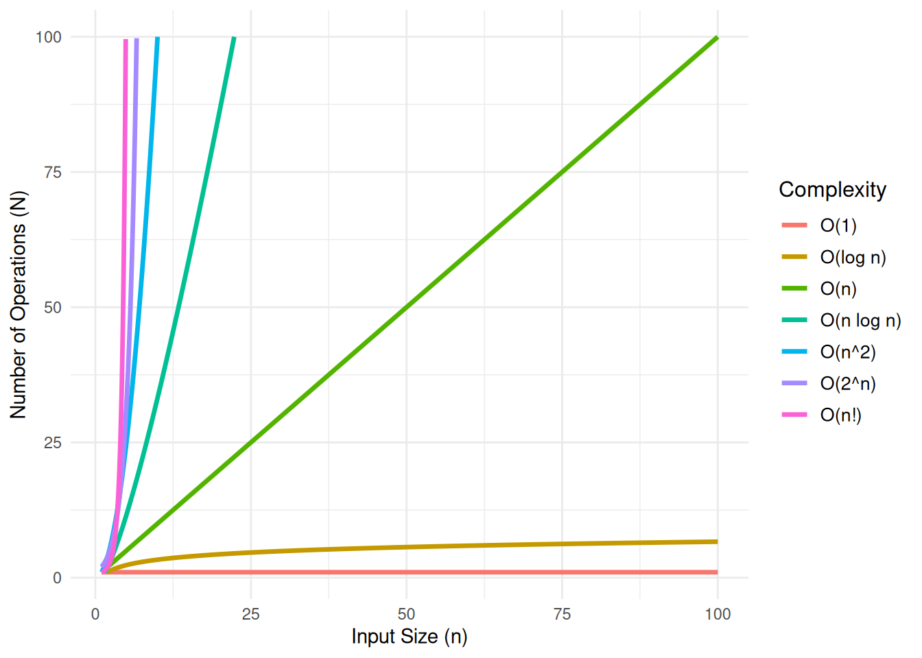
In theoretical computer science, the time complexity is the computational complexity that describes the amount of computer time it takes to run an algorithm. In the plot below, $n$ represents the size of the input, and $N$ represents the number of operations the algorithm performs. This relationship is a critical factor in defining the algorithm's performance, as the efficiency of the algorithm can be assessed by how $N$ changes as the input size $n$ increases.
[Learn more](https://en.wikipedia.org/wiki/Time_complexity){target="_blank"}
:::
```{r, warning=FALSE}
#| fig-cap: "Compirison of Computational Complexity"
#| fig-subcap: "It is good to know if the algorithm can handle my problem well!"
#| fig-alt: "A line plot of Computational Complexity"
library(data.table)
library(ggplot2)

# Seq `n` gen
n <- seq(0, 100, by = 0.01)  # need to make the increment small in order to avoid `Inf`s

# data.table
df <- data.table(
                  n = n,
                  `O(1)` = 1,
                  `O(log n)` = log2(n),
                  `O(n)` = n,
                  `O(n log n)` = n * log2(n),
                  `O(n^2)` = n^2,
                  `O(2^n)` = 2^n,
                  `O(n!)` = factorial(n)
                )

df_long <- data.table::melt(df, id.vars = "n", variable.name = "Complexity", value.name = "Time")

ggplot(df_long, aes(x = n, y = Time, color = Complexity)) +
      geom_line(size = 1.2) +
            ylim(1, 100) +
            xlim(1, 100)+
      labs(
            #title = "Compirison of Computational Complexity",
            x = "Input Size (n)",
            y = "Number of Operations (N)",
            color = "Complexity"
          ) +
      theme_minimal() +
      theme(
            plot.title = element_text(size = 16, face = "bold"),
            legend.title = element_text(size = 12),
            legend.text = element_text(size = 10)
      )
```
# Appendix
## Using Other Languages in Quarto
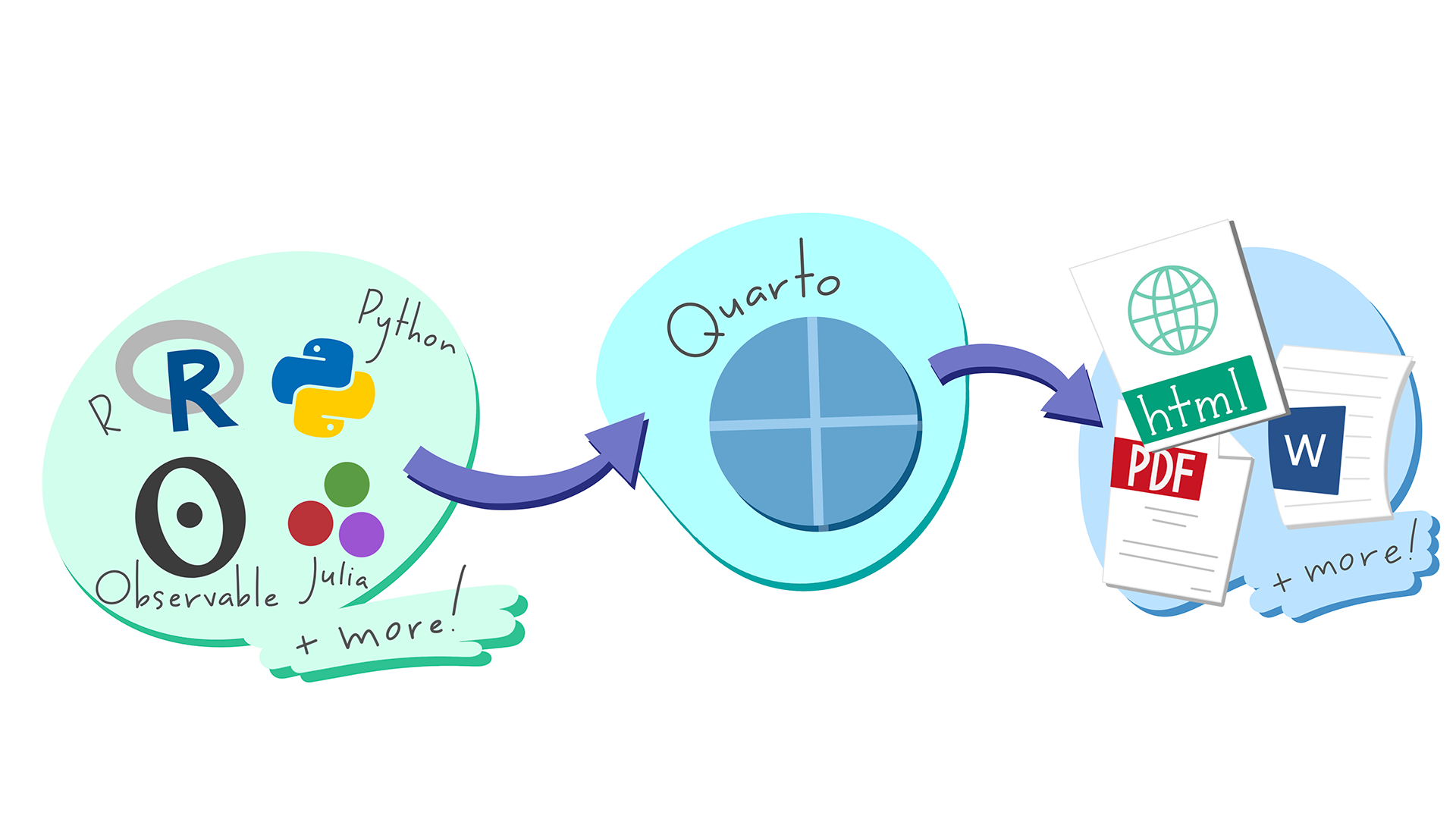
`Quarto` is a *language-agnostic publishing system* designed to integrate multiple computational engines. By using `{python}` blocks, researchers can execute `Python` code natively alongside R and Markdown.
Technical Mechanisms:
* Execution Engines: Depending on your setup, `Quarto` utilizes the Jupyter engine for `Python`-centric projects or the `Knitr` engine (via the `reticulate` package) for hybrid `R`-`Python` workflows.
* **Interoperability**: In a hybrid environment, data frames and variables can be shared between `R` and `Python` sessions, allowing you to use the best tools from both ecosystems (e.g., `Python` for machine learning and `R` for spatial statistics).
* Reproducibility: Consolidating multiple languages into **a single** `.qmd` file ensures that the entire analytical pipeline is documented and reproducible, regardless of the underlying programming language.
1. `R`
```{r}
print_a <- function(a) {
  a <- 1
  print(paste("Inside function:", a))
}
```
2. `Python`
```{python}

def print_a(a):

    a = 1
    print(f"Inside function: {a}")

```
3. `Julia`
```{julia}

function print_a(a)
    println("Inside function: $a")
end

```
```{fortran}

subroutine printA(A)
    implicit none

    integer, intent(in) :: A

    print*, "The value is:", A

end subroutine printA


```
### Reticulate (Python)
```{r}
library(reticulate)

#' Configure Python environment
#' Windows: Check for existing environment, create if missing, then bind.

env_name <- "quarto_demo"
py_ver <- "3.11"
py_lib <- c("scikit-learn", "pandas", "numpy", "scipy")


if (Sys.info()[["sysname"]] == "Windows") {

  # 1. Check if the environment exists in the conda list
  # We use name matching for robustness
  existing_envs <- conda_list()$name

  if (!(env_name %in% existing_envs)) {

    message("Environment '", env_name, "' not found. Creating environment...")
    # Create environment with specified python version
    conda_create(env_name, python_version = py_ver)

    # Install required packages after creation
    conda_install(env_name, packages = py_lib)
  } else {
    message("Environment '", env_name, "' already exists. Skipping creation.")
  }

  # 2. Bind to the environment
# use_condaenv requires the environment name (string), which is robust for Windows
  use_condaenv(env_name, required = TRUE)

} else {

  #' Linux (CI/CD): Setup baseline using micromamba (due to its ephemeral traits).
  # GitHub Actions / Linux Environment: Always fresh setup
  message("Linux/CI environment detected. Setting up baseline via micromamba...")
  py_lib_str <- paste(py_lib, collapse = " ")

  # Use 'micromamba create' instead of 'install' for a clean setup
  # -n: environment name
  # -c: channel specification
  # -y: automatic yes to prompts

  mamba_cmd <- sprintf("micromamba create -n %s -c conda-forge %s python=%s -y",
                       env_name, py_lib_str, py_ver)

  system(mamba_cmd)

  linux_env_path <- sprintf("/home/runner/micromamba/envs/%s/bin/python", env_name)
  use_condaenv(linux_env_path, required = TRUE)
}

# Verification of the loaded Python configuration
# print(py_config())


sys <- import("sys")

sys$executable
```
#### **Compairing Mathematical Foundations: OLS & MLE** {-}
In linear regression, we model the relationship between a dependent variable and independent variables as:
$$y = X\beta + \epsilon$$
Where the dimensions (shapes) are:
* $y \in \mathbb{R}^{N \times 1}$: Dependent variable vector.
* $X \in \mathbb{R}^{N \times K}$: Design matrix (including a column of 1s for the intercept).
* $\beta \in \mathbb{R}^{K \times 1}$: Parameter (coefficient) vector.
* $\epsilon \in \mathbb{R}^{N \times 1}$: Error (residual) vector.
::: {.panel-tabset}
#### OLS Perspective: Minimizing the SSR
The Ordinary Least Squares (OLS) method seeks to find $\beta$ that minimizes the Sum of Squared Residuals ($SSR$):
$$SSR(\beta) = \epsilon^T \epsilon = (y - X\beta)^T (y - X\beta)$$
##### **Matrix Expansion Steps** {-}
To derive the optimal $\beta$, we expand the expression using matrix algebra properties using following steps.
1. Distribution of Transpose
Using the rules $(A - B)^T = A^T - B^T$ and $(AB)^T = B^T A^T$:
$$(y - X\beta)^T = y^T - (X\beta)^T = y^T - \beta^T X^T$$
2. FOIL Expansion
Now we multiply $(y^T - \beta^T X^T)$ by $(y - X\beta)$:
$$SSR(\beta) = y^T y - y^T X \beta - \beta^T X^T y + \beta^T X^T X \beta$$
3. The Scalar Property (Merging Terms)
Note that $y^T X \beta$ is a scalar ($1 \times 1$). Any scalar is equal to its own transpose ($a = a^T$):
$$(y^T X \beta)^T = \beta^T X^T (y^T)^T = \beta^T X^T y$$
Since they are identical values, we can combine the middle terms:
$$SSR(\beta) = y^T y - 2\beta^T X^T y + \beta^T X^T X \beta$$
##### **The Normal Equation** {-}
Taking the partial derivative with respect to $\beta$:
$$\frac{\partial SSR}{\partial \beta} = -2X^T y + 2X^T X \beta = 0$$
Solving for $\beta$ gives the Normal Equation:
$$\hat{\beta}_{OLS} = (X^T X)^{-1} X^T y$$
#### MLE Perspective: Maximum Likelihood
Maximum Likelihood Estimation (MLE) assumes the errors follow a normal distribution: $\epsilon \sim \mathcal{N}(0, \sigma^2 I)$. The Log-Likelihood function is:
$$\mathcal{L}(\beta, \sigma^2) = -\frac{N}{2}\ln(2\pi\sigma^2) - \frac{1}{2\sigma^2} \sum_{i=1}^{N} (y_i - X_i\beta)^2$$
In MLE, maximizing $\mathcal{L}$ with respect to $\beta$ is identical to minimizing the summation term $\sum (y_i - X_i\beta)^2$, which is exactly the $SSR$ used in OLS. Thus, under *Gaussian* assumptions, **OLS and MLE are mathematically equivalent**.
:::
#### Implementation: R and Python Interoperability
We use the 'meuse' soil dataset from the sp package to verify this equivalence.
##### Data Preparation (R)
We use the 'meuse' soil dataset. We will predict Zinc concentration ($y$) using Copper concentration ($x$).
```{r}
#| label: data-preparation
library(sp)
library(reticulate)

# Load Meuse dataset
data(meuse)

# Prepare Design Matrix X (adding an intercept column of 1s) and Target Vector y
y_vec <- as.matrix(meuse$zinc)
x_mat <- as.matrix(cbind(1, meuse$copper))

cat("Number of observations (N):", nrow(x_mat), "\n")
```
##### Matrix Algebra & Optimization (Python)
We will perform both OLS (via linear algebra) and MLE (via numerical optimization) explicitly in Python to demonstrate their equivalence.
We use NumPy for the direct linear algebra solution (OLS) and SciPy for numerical optimization (MLE).
```{python}
#| label: python-ols-mle
import numpy as np
from scipy.optimize import minimize

# 1. Retrieve variables from R environment
X = r.x_mat
y = r.y_vec
N = X.shape[0]

# =========================================================
# Step 1: Ordinary Least Squares (OLS) via Linear Algebra
# =========================================================
def compute_ols(X_matrix: np.ndarray, y_vector: np.ndarray) -> np.ndarray:
    """
    Compute OLS coefficients using the Normal Equation.

    Args:
        X_matrix (np.ndarray): Design matrix.
        y_vector (np.ndarray): Target vector.

    Returns:
        np.ndarray: Beta coefficients.
    """
    xtx = X_matrix.T @ X_matrix
    xty = X_matrix.T @ y_vector
    return np.linalg.solve(xtx, xty)

beta_ols = compute_ols(X, y)

print("--- 1. OLS Results (NumPy Linear Algebra) ---")
print(f"Intercept: {beta_ols[0][0]:.4f}")
print(f"Slope (Copper): {beta_ols[1][0]:.4f}\n")
# =========================================================
# Step 2: Maximum Likelihood Estimation (MLE) via Optimization
# =========================================================
def negative_log_likelihood(params: np.ndarray) -> float:
    """
    Calculate the Negative Log-Likelihood for a Gaussian regression model.

    Args:
        params (np.ndarray): Array containing [intercept, slope, variance].

    Returns:
        float: The NLL value to be minimized.
    """
    beta = params[0:2].reshape(-1, 1)
    variance = params[2]

    # Mathematical constraint: Variance must be strictly positive
    if variance <= 0:
        return np.inf

    # Calculate Sum of Squared Residuals (SSR)
    residuals = y - (X @ beta)
    ssr = np.sum(residuals ** 2)

    # Calculate NLL formula
    nll = (N / 2) * np.log(2 * np.pi * variance) + (ssr / (2 * variance))
    return float(nll)

# Initial guess for the optimizer: [intercept=0, slope=0, variance=10]
initial_guess = np.array([0.0, 0.0, 10.0])

# Run L-BFGS-B optimization algorithm to find the MLE parameters
mle_result = minimize(negative_log_likelihood, initial_guess, method='L-BFGS-B')

beta_mle = mle_result.x[0:2]
variance_mle = mle_result.x[2]

print("--- 2. MLE Results (SciPy Optimization) ---")
print(f"Intercept: {beta_mle[0]:.4f}")
print(f"Slope (Copper): {beta_mle[1]:.4f}")
print(f"Estimated Variance: {variance_mle:.4f}\n")
# =========================================================
# Step 3: Verify Mathematical Equivalence
# =========================================================
diff = np.abs(beta_ols.flatten() - beta_mle)
print("--- 3. Equivalence Check (Difference |OLS - MLE|) ---")
print(f"Difference in Intercept: {diff[0]:.2e}")
print(f"Difference in Slope: {diff[1]:.2e}")
```
##### Verification with R's Native Function (R)
Finally, we verify that our explicit matrix operations match R's default statistical engine.
```{r}
#| label: r-verification
# Fit OLS using R's built-in linear model function
r_lm <- lm(zinc ~ copper, data = meuse)

cat("--- R's lm() Coefficients ---\n")
print(coef(r_lm))
```
::: {.callout-note}
## Why OLS and MLE results differ: Numerical Approximation Error
While OLS and MLE are theoretically identical for linear regression with normally distributed errors, you may observe slight discrepancies in your output (e.g., ~0.006 in slope). This is called **Approximation Error**.
**Exact vs. Iterative Solutions**
- **OLS (Analytical):** Uses a "Closed-form Solution" ($\hat{\beta} = (X^TX)^{-1}X^Ty$). It calculates the exact mathematical global minimum in a single step using matrix algebra.
- **MLE (Numerical):** Uses "Numerical Optimization" (e.g., BFGS algorithm in `scipy.optimize`). It "hunts" for the maximum likelihood by taking iterative steps until it reaches a pre-defined threshold.
:::
------------------------------------------------------------------------
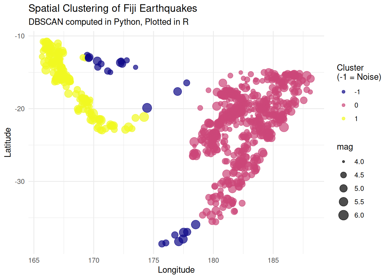
#### **DataFrame Operations: Spatial Point Clustering (R $\rightarrow$ Python $\rightarrow$ R)** {-}
This is a pipeline that transfers seismic event location data (`quakes`) from `R` to `Python` to perform Density-Based Spatial Clustering of Applications with Noise (DBSCAN), then brings the results back to `R` for final visualization.
**Objective Evaluation:** In spatial pattern analysis, `scikit-learn`'s DBSCAN implementation is highly optimized at the C/C-Python level, offering significantly faster processing speeds for point clouds with hundreds of thousands of points compared to standard R packages. This architecture establishes an ideal division of labor: Python handles the heavy computational load, while R’s `ggplot2` produces high-quality visualizations suitable for publication.
```{r}
#| label: load-spatial-points
# Load built-in Fiji earthquakes dataset
data(quakes)

# Select spatial coordinates and magnitude
spatial_df <- quakes[, c("lat", "long", "mag")]
head(spatial_df, 3)
```
```{python}
#| label: python-clustering
import pandas as pd
from sklearn.cluster import DBSCAN

def perform_spatial_clustering(df: pd.DataFrame, eps: float = 2.0, min_samples: int = 15) -> np.ndarray:
    """
    Apply DBSCAN clustering algorithm to spatial coordinates.

    Args:
        df (pd.DataFrame): DataFrame containing 'lat' and 'long' columns.
        eps (float): The maximum distance between two samples for one to be considered
                     as in the neighborhood of the other.
        min_samples (int): The number of samples in a neighborhood for a point
                           to be considered as a core point.

    Returns:
        np.ndarray: Array of cluster labels (-1 indicates noise).
    """
    # Extract coordinates as a NumPy array
    coords = df[['lat', 'long']].values

    # Initialize and fit DBSCAN
    clustering_model = DBSCAN(eps=eps, min_samples=min_samples)
    labels = clustering_model.fit_predict(coords)

    return labels

# r.spatial_df is automatically converted to a Pandas DataFrame
cluster_labels = perform_spatial_clustering(r.spatial_df)
```
```{r}
#| label: plot-clusters
library(ggplot2)

# Bind the Python-generated labels back to the R dataframe
spatial_df$cluster <- as.factor(py$cluster_labels)

# Generate publication-ready plot
ggplot(spatial_df, aes(x = long, y = lat, color = cluster, size = mag)) +
  geom_point(alpha = 0.7) +
  scale_color_viridis_d(option = "plasma", name = "Cluster\n(-1 = Noise)") +
  theme_minimal() +
  labs(
    title = "Spatial Clustering of Fiji Earthquakes",
    subtitle = "DBSCAN computed in Python, Plotted in R",
    x = "Longitude",
    y = "Latitude"
  )
```
### Observable JS (Client-side Interactivity)
While R and Python are excellent for heavy data processing, **Observable JavaScript (OJS)** is optimized for building real-time, interactive visualizations directly in the user's web browser.
Quarto bridges these two environments using the `ojs_define()` function. The standard workflow is:
1. Process large datasets in R during the build phase.
2. Export the aggregated data to OJS.
3. Render interactive plots in the browser without needing an active R server.
#### Step A: Data Processing in R {-}
```{r}
#| message: false
#| warning: false
library(data.table)

# 1. Generate sample environmental data (e.g., temperature across stations)
set.seed(42)
dt_env <- data.table(
  station = rep(c("Station_A", "Station_B", "Station_C"), each = 50),
  day = rep(1:50, 3),
  temperature = c(rnorm(50, 15, 2), rnorm(50, 18, 3), rnorm(50, 12, 1.5))
)

# 2. Export the data to the Observable JS environment
ojs_define(env_data = dt_env)
```
#### Step B: Interactive Plotting in Observable JS {-}
In the following `ojs` chunk, we take the data processed by R and create an interactive plot. Try changing the dropdown menu to filter the stations in real-time.
```{ojs}
//| echo: true
//| code-fold: false
// 1. Transpose the data (R data frames become column-major JSON arrays, OJS needs row-major)
data = transpose(env_data)

// 2. Create a reactive dropdown input
viewof selected_station = Inputs.select(
  ["Station_A", "Station_B", "Station_C"],
  {label: "Select Station:"}
)

// 3. Filter data based on user selection
filtered_data = data.filter(d => d.station === selected_station)

// 4. Render the plot using Observable Plot
Plot.plot({
  y: {
    grid: true,
    label: "Temperature (°C)"
  },
  x: {
    label: "Day of Observation"
  },
  marks: [
    Plot.line(filtered_data, {x: "day", y: "temperature", stroke: "steelblue", strokeWidth: 2}),
    Plot.dot(filtered_data, {x: "day", y: "temperature", fill: "black"})
  ]
})
```
```{r}
if (Sys.info()[[1]]=="Windows") {

    # For my Windows Environment
    system("systeminfo",intern = T)

    } else{

    system("lscpu; free -h",intern = T)


}
```
<!-- # Clean-up {-} -->
<!-- ```{r} -->
<!-- remove_python_env(env_name) -->
<!-- ``` -->