1 Intro - Backdrop

This example demonstrates how Quarto documents can be rendered in GitHub-Actions CI/CD environment with the required Python/R package dependencies. This need pre-setup - see: my .github/workflows and GitHub Actions for more details.

The code below is part of what I used for my Master’s thesis. In my thesis, I used the binary data provided from Korea Meteorological Agency(KMA) which contains radar reflectance of precipitation. Using the code below, I derived the rainfall intensity and the amount of antecedent rainfall and plugged them into my machine learning models.

2 Setup Reticulate

I am kinda R person and not a big fan of python(because of the indentation… You know… hard to do for loops and if statements), but I had no choice but use Python because I needed the greatest package of all time, i.e., NumPy for handling multidimensional array. Also, the handling of binary data sucks in R made me to use it.

Code

library(reticulate)



if (Sys.info()[[1]]=="Windows") {
        
    # For my Windows Environment
    use_condaenv("C:\\Users\\dydgn\\anaconda3\\envs\\baseline\\python.exe", required = TRUE)    
    
    } else{
    
    # For github actions to utilize CI/CD
    use_condaenv("/home/runner/micromamba/envs/baseline/bin/python", required = TRUE)   
    
}

3 The First step with Python

3.1 Import Some Packages

Code

import sys
print(sys.executable)

/home/runner/micromamba/envs/baseline/bin/python

This will show where the python executable binary is.

Code

import numpy as np
import matplotlib.pyplot as plt
import os
import struct
import gzip

Importing basic packages

3.2 Handling Various File Formats

3.2.1 Get the Size of a Compressed Gunzip, i.e., Raw File

Code

file = "./data/RDR_HSR_22_20220808/RDR_CMP_HSR_PUB_202208082200.bin.gz"



# # Get the size of the binary data file in bytes
file_size = os.path.getsize(file)

print("The compressed data file size is {} bytes.".format(file_size))

The compressed data file size is 608837 bytes.

3.2.2 Get the Size of a Binary file

Code

def getuncompressedsize(filename):
    with open(filename, 'rb') as f:
        f.seek(-4, 2)
        return struct.unpack('I', f.read(4))[0]

file_size = getuncompressedsize(file)

print("The binary data file size is {} bytes.".format(file_size))

The binary data file size is 13282434 bytes.

3.3 Hmm.. Do you know how to cook a binary file?

I had to read the manual provided to convert a binary file into so-called raster

3.3.1 Read a binary as a numpy array

Code

header_size = 1024


# Check if the file size is non-zero
if file_size == 0:
    print("The binary data file is empty.")
else:
  f = gzip.GzipFile(file)
  f.seek(header_size)
  file_content = f.read()
  data = np.frombuffer(file_content, dtype=np.short)
  f.close()

3.3.2 Reshape the array using the number from the official manual

Code

# Reshape the data into a 2D array
data = data.reshape(2881, 2305)
# data needs to be flipped!
data = np.flipud(data)

data.shape

(2881, 2305)

3.3.3 Initial plotting

Code

#### Plotting

def matplot(x):
  
  plt.clf()
  plt.imshow(x)
  plt.colorbar()
  plt.show()


matplot(data)

3.3.4 Munging data

To use as a feature of the model, I had to change the radar reflectance into the amount of rainfall intensity by using Z-R relationship.

Code


# Scale factor

#define PUB_OUT   -30000 // Outside of the observed region

#define PUB_IN    -25000 // Unobserved areas within the observed region

#define PUB_MIN   -20000 // Minimum value for representation within the observed area


data = np.where(data<-20000, 0, data)

echo = data*0.01




# Z-R Relation

ZRa = 148.

ZRb = 1.59

# converting dBZ to rain

def dbz2rain(x):

    rain = (x*0.1 - np.log10(ZRa))/ZRb

    rain = 10**rain

    return rain


R = dbz2rain(echo)

R[R<=0.04315743] = 0.0

After the conversion, then we get the actual amount of rainfall intensity in mm/hr.

Code

# Unit: millimeter per hour

matplot(R)

4 Back to the R environment!

4.1 Plot using raster::plot()

Code

#handy R-python interface: reticulate

pcp <- py$R

library(raster)

Loading required package: sp

Code

test <- raster(pcp,
       xmn=(-1121*500),
       xmx=((2305-1121)*500),
       ymn=(-1681*500),
       ymx=(2881-1681)*500,
       crs = CRS("+proj=lcc +lat_1=30 +lat_2=60 +lat_0=38 +lon_0=126 +a=6378138.00 +b=6356752.314 +units=m +no_defs")
       )


plot(test)

4.2 Plot using tmap package

Code

library(tmap)

Breaking News: tmap 3.x is retiring. Please test v4, e.g. with
remotes::install_github('r-tmap/tmap')

Code

library(leafem)

tmap_mode("view")

tmap mode set to interactive viewing

Code

test[test==0]=NA

{
  tm_basemap(c("OpenStreetMap.HOT",
               "https://mt1.google.com/vt/lyrs=y&hl=en&z={z}&x={x}&y={y}",
               "https://mt1.google.com/vt/lyrs=s&hl=en&z={z}&x={x}&y={y}"),
             group = list(c("OpenStreetMap.HOT",
                       "Google Satellite Imagery w/ label",
                       "Google Satellite Imagery wo/ label"))) +
    tm_shape(test)  +                                  
    tm_raster(title = "Max Rainfall Intensity[mm/hr]",
              palette = "-Spectral",
              style = "cont") -> themap
  
  
  
  tmap_leaflet(themap)|>
    addMouseCoordinates()
  
}

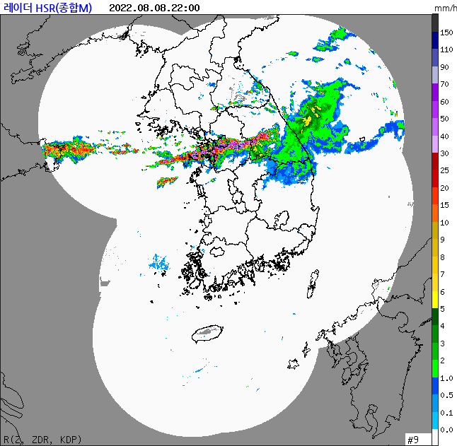
stars object downsampled to 895 by 1118 cells. See tm_shape manual (argument raster.downsample)

4.2.1 Extra: Compairing with the plot from Korea Meteorological Agency

--- title: "Python Dependency Test" subtitle: "Test Case of Handling a Binary Data with Python" author: "Yonghun Suh" date: "Oct 9, 2024" categories: [Code] image: https://db0dce98.rocketcdn.me/en/files/2020/04/Diapositive1-1.png format: html: toc: true number_sections: true code-copy: true code-fold: show code-tools: true code-overflow: scroll code-link: true number-sections: true toc_depth: 3 lightbox: true #execute: # freeze: true #comments: false --- # Intro - Backdrop This example demonstrates how Quarto documents can be rendered in GitHub-Actions **CI/CD** environment with the required Python/R package dependencies. This need pre-setup - see: [my `.github/workflows`](https://github.com/YONGHUNI/blog/tree/main/.github/workflows){target="_blank"} and [GitHub Actions](https://github.com/features/actions){target="_blank"} for more details. The code below is part of what I used for my Master's thesis. In my thesis, I used the binary data provided from Korea Meteorological Agency(KMA) which contains radar reflectance of precipitation. Using the code below, I derived the rainfall intensity and the amount of antecedent rainfall and plugged them into my machine learning models. # Setup Reticulate I am kinda `R` person and not a big fan of python(because of the indentation... You know... hard to do `for` loops and `if` statements), but I had no choice but use `Python` because I needed the greatest package of all time, *i.e.*, `NumPy` for handling multidimensional array. Also, the handling of binary data sucks in R made me to use it. ```{r} library(reticulate) if (Sys.info()[[1]]=="Windows") { # For my Windows Environment use_condaenv("C:\\Users\\dydgn\\anaconda3\\envs\\baseline\\python.exe", required = TRUE) } else{ # For github actions to utilize CI/CD use_condaenv("/home/runner/micromamba/envs/baseline/bin/python", required = TRUE) } ``` # The First step with Python ## Import Some Packages ```{python} import sys print(sys.executable) ``` This will show where the python executable binary is. ```{python} import numpy as np import matplotlib.pyplot as plt import os import struct import gzip ``` Importing basic packages ## Handling Various File Formats ### Get the Size of a Compressed Gunzip, **i.e.,** Raw File ```{python} file = "./data/RDR_HSR_22_20220808/RDR_CMP_HSR_PUB_202208082200.bin.gz" # # Get the size of the binary data file in bytes file_size = os.path.getsize(file) print("The compressed data file size is {} bytes.".format(file_size)) ``` ### Get the Size of a Binary file ```{python} def getuncompressedsize(filename): with open(filename, 'rb') as f: f.seek(-4, 2) return struct.unpack('I', f.read(4))[0] file_size = getuncompressedsize(file) print("The binary data file size is {} bytes.".format(file_size)) ``` ## Hmm.. Do you know how to cook a binary file? I had to read the manual provided to convert a binary file into so-called `raster` ```{r, echo=FALSE, out.width="100%", out.height=600, fig.align = "center"} knitr::include_graphics("./data/manual/레이더 합성자료 포맷 정의서_외부제공용.pdf") ``` ### Read a binary as a numpy array ```{python} header_size = 1024 # Check if the file size is non-zero if file_size == 0: print("The binary data file is empty.") else: f = gzip.GzipFile(file) f.seek(header_size) file_content = f.read() data = np.frombuffer(file_content, dtype=np.short) f.close() ``` ### Reshape the array using the number from the official manual ```{python} # Reshape the data into a 2D array data = data.reshape(2881, 2305) # data needs to be flipped! data = np.flipud(data) data.shape ``` ### Initial plotting ```{python} #### Plotting def matplot(x): plt.clf() plt.imshow(x) plt.colorbar() plt.show() matplot(data) ``` ### Munging data To use as a feature of the model, I had to change the radar reflectance into the amount of rainfall intensity by using [Z-R relationship](https://www.scirp.org/journal/paperinformation?paperid=71153){target="_blank"}. ```{python} # Scale factor #define PUB_OUT -30000 // Outside of the observed region #define PUB_IN -25000 // Unobserved areas within the observed region #define PUB_MIN -20000 // Minimum value for representation within the observed area data = np.where(data<-20000, 0, data) echo = data*0.01 # Z-R Relation ZRa = 148. ZRb = 1.59 # converting dBZ to rain def dbz2rain(x): rain = (x*0.1 - np.log10(ZRa))/ZRb rain = 10**rain return rain R = dbz2rain(echo) R[R<=0.04315743] = 0.0 ``` After the conversion, then we get the actual amount of rainfall intensity in `mm/hr`. ```{python} # Unit: millimeter per hour matplot(R) ``` # Back to the R environment! ## Plot using raster::plot() ```{r} #handy R-python interface: reticulate pcp <- py$R library(raster) test <- raster(pcp, xmn=(-1121*500), xmx=((2305-1121)*500), ymn=(-1681*500), ymx=(2881-1681)*500, crs = CRS("+proj=lcc +lat_1=30 +lat_2=60 +lat_0=38 +lon_0=126 +a=6378138.00 +b=6356752.314 +units=m +no_defs") ) plot(test) ``` ## Plot using tmap package ```{r} library(tmap) library(leafem) tmap_mode("view") test[test==0]=NA { tm_basemap(c("OpenStreetMap.HOT", "https://mt1.google.com/vt/lyrs=y&hl=en&z={z}&x={x}&y={y}", "https://mt1.google.com/vt/lyrs=s&hl=en&z={z}&x={x}&y={y}"), group = list(c("OpenStreetMap.HOT", "Google Satellite Imagery w/ label", "Google Satellite Imagery wo/ label"))) + tm_shape(test) + tm_raster(title = "Max Rainfall Intensity[mm/hr]", palette = "-Spectral", style = "cont") -> themap tmap_leaflet(themap)|> addMouseCoordinates() } ``` ### Extra: Compairing with the plot from Korea Meteorological Agency ![](data/RDR_CMI_202208082200.png)