---
title: "How to boost a DBSCAN task"
subtitle: "Utilizing High Performance Library from Python"
author: "Yonghun Suh"
date: "Sep. 9, 2025"
categories: [Code]
image: https://raw.githubusercontent.com/wangyiqiu/dbscan-python/0.0.12-dev/compare.png
format:
html:
toc: true
number_sections: true
code-copy: true
code-fold: show
code-tools: true
code-overflow: scroll
code-link: true
number-sections: true
toc_depth: 3
lightbox: true
#execute:
# freeze: true
#comments: false
---
# Backdrop
{width=70%}
>[Frodo, 2:37 PM] I'm working on finding representative points for census tracts using nationwide residential building data, weighted by the population of each tract.<br>
[Frodo, 2:38 PM] But DBSCAN is taking forever lol, so I'm running it in parallel.<br>
[Frodo, 2:38 PM] Using something like the future package in R.<br>
[Yong-Hun Suh, 2:41 PM] Yeah, DBSCAN’s time complexity isn’t great…<br>
[Yong-Hun Suh, 4:47 PM] Are you still working on that (DBSCAN)?<br>
[Yong-Hun Suh, 4:47 PM] If it’s a project you’re going to continue, I can give you a tip…<br>
[Frodo, 4:53 PM] Just fixed the code and running it now haha, results should come out in a **few days** if it’s fast.<br>
I was chatting with my colleague from grad school who said DBSCAN was running too slowly on their project.
He had already been using a high speed C++ implementation of DBSCAN in R. Still, however, it was giving an eternal waiting.
I thought, 'Why not help him out and turn this into a blog article?'
## **Analyzing complexity factors**
::: {.callout-tip}
## What is Time Complexity?
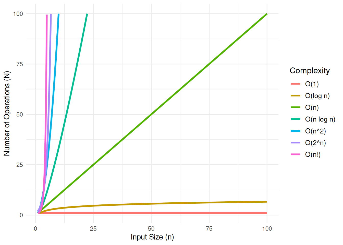
In theoretical computer science, the time complexity is the computational complexity that describes the amount of computer time it takes to run an algorithm. In the plot below, $n$ represents the size of the input, and $N$ represents the number of operations the algorithm performs. This relationship is a critical factor in defining the algorithm's performance, as the efficiency of the algorithm can be assessed by how $N$ changes as the input size $n$ increases.
[Learn more](https://en.wikipedia.org/wiki/Time_complexity){target="_blank"}
:::
```{r, warning=FALSE}
#| fig-cap: "Compirison of Computational Complexity"
#| fig-subcap: "It is good to know if the algorithm can handle my problem well!"
#| fig-alt: "A line plot of Computational Complexity"
library(data.table)
library(ggplot2)

# Seq `n` gen
n <- seq(0, 100, by = 0.01)  # need to make the increment small in order to avoid `Inf`s

# data.table
df <- data.table(
                  n = n,
                  `O(1)` = 1,
                  `O(log n)` = log2(n),
                  `O(n)` = n,
                  `O(n log n)` = n * log2(n),
                  `O(n^2)` = n^2,
                  `O(2^n)` = 2^n,
                  `O(n!)` = factorial(n)
                )

df_long <- data.table::melt(df, id.vars = "n", variable.name = "Complexity", value.name = "Time")

ggplot(df_long, aes(x = n, y = Time, color = Complexity)) +
      geom_line(size = 1.2) +
            ylim(1, 100) +
            xlim(1, 100)+
      labs(
            #title = "Compirison of Computational Complexity",
            x = "Input Size (n)",
            y = "Number of Operations (N)",
            color = "Complexity"
          ) +
      theme_minimal() +
      theme(
            plot.title = element_text(size = 16, face = "bold"),
            legend.title = element_text(size = 12),
            legend.text = element_text(size = 10)
      )
```
## DBSCAN time complexity
DBSCAN’s runtime is dominated by how you perform neighborhood (range) queries. The classic “it’s $O(n²)$” is only the worst case of a spectrum that depends on data distribution, dimensionality, the index used, and the radius parameter $\varepsilon$.
---
### Core steps and cost drivers
- **Range queries:** For each point, find all neighbors within radius $\varepsilon$. Distance evaluation for one pair costs $O(d)$ in $d$-dimensional Euclidean space.
- **Cluster expansion:** A queue-based flood-fill that repeatedly issues range queries starting from core points (points with at least $\text{minPts}$ neighbors within $\varepsilon$).
Asymptotically, the number and cost of range queries dominate; the expansion logic is linear in the number of discovered neighbors but tied to the same range-query results.
---
### Complexity by neighborhood search strategy
#### Brute-force (no index)
- Per range query: compute distance to all points ⇒ $O(n \cdot d)$.
- One query per point in the simplest implementation ⇒ $O(n^2 \cdot d)$.
- Cluster expansion may reuse queries or cause repeats; asymptotically the bound remains $\Theta(n^2 \cdot d)$ in the worst case.
#### Space-partitioning trees (kd-tree, ball tree, R-tree-like)
- Index build: typically $O(n \log n)$ time, $O(n)$ space.
- Range query cost:
- Best/average (well-behaved low–moderate $d$, balanced tree, moderate $\varepsilon$): $O(\log n + k)$, where $k$ is the number of reported neighbors.
- Worst case (high $d$, large $\varepsilon$, or adversarial data): degenerates to $O(n)$.
- Overall:
- Best/average: $O(n \log n + \sum \limits_{i=1}^{n} (\log n + k_i)) = O(n \log n + K)$, where $K = \sum k_i$ is total neighbor reports. If density per query is bounded, $K = O(n)$, giving $O(n \log n)$ plus distance cost factor $O(d)$.
- Worst: $O(n^2 \cdot d)$.
#### Uniform grid (fixed-radius hashing) in low dimensions
- Build grid hashing once: expected $O(n)$.
- Range query: constant number of adjacent cells, expected $O(1 + k)$ in 2D/3D if $\varepsilon$ is aligned with cell size and data are not pathologically skewed.
- Overall in practice: near-linear $O(n + K)$, again with distance cost $O(d)$, but this approach becomes brittle as $d$ grows.
> In all cases, include the distance computation factor $O(d)$. For high dimensions, tree and grid pruning effectiveness collapses, pushing complexity toward $\Theta(n^2 \cdot d)$.
---
## What influences the runtime
- **Dimensionality $d$:** Distance costs scale with $O(d)$, and index pruning degrades with the curse of dimensionality, often turning tree queries into $O(n)$.
- **Neighborhood radius $\varepsilon$:** Larger $\varepsilon$ increases average neighbor count $k$, raises $K=\sum k_i$, and triggers more expansions; in the limit, most points neighbor each other ⇒ near $O(n^2 \cdot d)$.
- **Data distribution and density:** Well-separated, roughly uniform, low-density data favor subquadratic performance with indexes. Dense clusters or large connected components increase expansions and repeats.
- **minPts:** Affects how many points become core (thus how much expansion occurs). It changes constants and practical behavior but not the worst-case big-O bound.
- **Distance metric:** Non-Euclidean metrics can alter pruning efficacy and per-distance cost.
- **Implementation details:** Caching of range queries, deduplication, and “expand only once per point” optimizations materially reduce constants.
---
## Practical scenarios
| Scenario | Assumptions | Typical complexity |
|---|---|---|
| Brute-force baseline | Any $d$, no index | $\Theta(n^2 \cdot d)$ |
| Tree index, low–moderate $d$ | Balanced tree, moderate $\varepsilon$, bounded neighbor counts | $O(n \log n \cdot d)$ |
| Tree index, high $d$ or large $\varepsilon$ | Poor pruning, dense neighborhoods | $\Theta(n^2 \cdot d)$ |
| Grid index (2D/3D) | Well-chosen cell size, non-pathological data | Near $O(n \cdot d)$ |
| Approximate NN/range | ANN structure (e.g., HNSW), approximate neighbors | Subquadratic wall-time; formal bounds vary |
::: {.callout-note}
- The index build cost $O(n \log n)$ (trees) or $O(n)$ (grid) is typically amortized across all range queries.
- If each point’s neighbor count $k_i$ is bounded by a small constant on average, and pruning works, the total neighbor reports $K$ is $O(n)$, leading to near $O(n \log n)$ behavior with trees.
:::
> But... What if you neither can reduce your dataset... nor change the parameter of the DBSCAN?
## Solution...? At least for this case :)
**Use more efficient algorithms that fully leverage your hardware's full potential!**
For this case, I used `dbscan-python`, which is a high-performance parallel implementation of DBSCAN, based on the SIGMOD 2020 paper “[Theoretically Efficient and Practical Parallel DBSCAN](https://github.com/wangyiqiu/dbscan-python){target="_blank"}.”
This work achieves theoretically-efficient clustering by minimizing total work and maintaining polylogarithmic parallel depth, enabling scalable performance on large datasets.
Compared to the naive $O(n^2)$ approach, the proposed algorithm reduces time complexity to $O(n \log n)$ work and $O(\log n)$ depth in 2D, and sub-quadratic work in higher dimensions through grid-based partitioning, parallel union-find, and spatial indexing techniques.
As the name of the package implies, I need to use Python again for this experiment.
# Experiments
## Setups
### Used R Packages
```{r warning=FALSE}
library(dbscan)
library(data.table)
library(arrow)
library(future.apply)
library(ggplot2)
```
### Python Setup
```{r}
library(reticulate)


if (Sys.info()[[1]]=="Windows") {

    # For my Windows Environment
    use_condaenv("C:/Users/dydgn/miniforge3/envs/dbscan/python.exe")

    } else{

    system("micromamba install -n baseline -c conda-forge dbscan -y")

    # For github actions to utilize CI/CD

    use_condaenv("/home/runner/micromamba/envs/baseline/bin/python", required = TRUE)


}


sys <- import("sys")

sys$executable
```
## Generated Lab Dataset
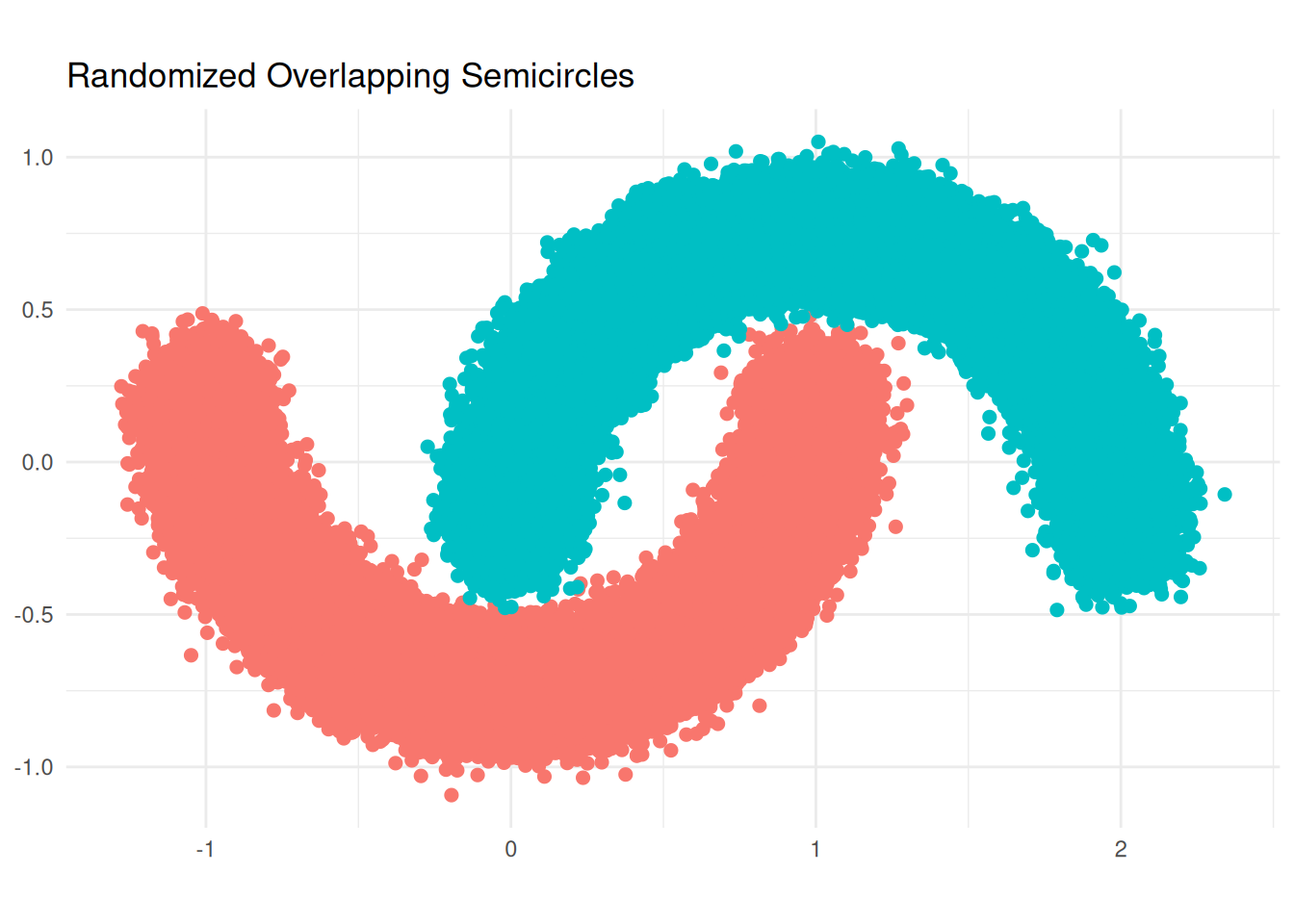
First, I had to replicate a famous dataset for demonstrating DBSCAN.
```{r}
generate_random_semicircle <- function(center_x, center_y, radius, start_angle, end_angle, n_points = 100, noise = 0.08) {

      angles <- runif(n_points, min = start_angle, max = end_angle)
      x <- center_x + radius * cos(angles) + rnorm(n_points, 0, noise)
      y <- center_y + radius * sin(angles) + rnorm(n_points, 0, noise)

      return(as.data.table(list(x = x, y = y)))
}


set.seed(123)


N <- 1e+5L


semicircle1 <- generate_random_semicircle(center_x = 0, center_y = 0.25, radius = 1,
                                          start_angle = pi, end_angle = 2 * pi, n_points = N)
semicircle1[, group := "Semicircle 1"]


semicircle2 <- generate_random_semicircle(center_x = 1, center_y = -0.25, radius = 1,
                                          start_angle = 0, end_angle = pi, n_points = N)
semicircle2[, group := "Semicircle 2"]


df <- rbindlist(list(semicircle1, semicircle2))


# visualization
ggplot(df, aes(x = x, y = y, color = group)) +
  geom_point(size = 2) +
  coord_fixed(ratio = 1) +
  theme_minimal() +
  labs(title = "Randomized Overlapping Semicircles", x = NULL, y = NULL) +
  theme(legend.position = "none")
lab_data <- df[, !c("group"), with = FALSE]
```
### R - Naive
```{r}
lab_data_r <- lab_data

epsilon <-  .08
minpts <- 200L #should be an integer for the python env


stime <- Sys.time()
db_result_r <- dbscan(lab_data_r, eps = epsilon, minPts = minpts)
etime <- Sys.time()

delta_t_r <- etime-stime; delta_t_r
# result
table(db_result_r$cluster)
lab_data_r$group <- as.factor(db_result_r$cluster)

# visualization
ggplot(lab_data_r, aes(x = x, y = y, color = group)) +
    geom_point(size = 2) +
    coord_fixed(ratio = 1) +
    theme_minimal() +
    labs(title = "Randomized Overlapping Semicircles", x = NULL, y = NULL) +
    theme(legend.position = "none")
```
### Python - `wangyiqiu/dbscan-python`
```{r}
lab_data_py <- lab_data

py$lab_data <- as.matrix(lab_data_py)
py$epsilon <- epsilon
py$minpts <- minpts
```
```{python}
import numpy as np
from dbscan import DBSCAN
import time

print("type(X):", type(lab_data))
print("shape(X):", getattr(lab_data, 'shape', None))
start = time.time()
labels, core_samples_mask = DBSCAN(lab_data, eps = epsilon, min_samples = minpts)
end = time.time()


delta_t = end - start

print(f"Elapsed time: {delta_t:.4f} seconds")
# 결과를 R로 반환
#r.labels = labels
#r.core_mask = core_samples_mask
```
```{r}
# result
table(py$labels)
lab_data_py$group <- as.factor(py$labels+1) # as index number starts from 0

# visualization
ggplot(lab_data_py, aes(x = x, y = y, color = group)) +
      geom_point(size = 2) +
      coord_fixed(ratio = 1) +
      theme_minimal() +
      labs(title = "Randomized Overlapping Semicircles", x = NULL, y = NULL) +
      theme(legend.position = "none")
```
### Results
```{r}
#speedup


cat(delta_t_r[[1]]/py$delta_t," times speed-up\n",sep = "")
```
## Some Real World Dataset
Source: [NYC Taxi Data](https://www.nyc.gov/site/tlc/about/tlc-trip-record-data.page)
```{r}
months <- 1

urls <- paste0("https://d37ci6vzurychx.cloudfront.net/trip-data/yellow_tripdata_2024-",sprintf("%02d", 1:months),".parquet")


plan(multisession,workers = 2)

taxi_list <- future_lapply(urls, function(url) as.data.table(read_parquet(url))) |> rbindlist()

gc()
head(taxi_list)
# select numeric rows & filtering out NAs
taxi_numeric_dt <- taxi_list[
    trip_distance > 0 & fare_amount > 0 & !is.na(trip_distance) & !is.na(fare_amount),
    .(trip_distance, fare_amount)
]

rm(taxi_list)
gc()
taxi_numeric_dt_200k <- taxi_numeric_dt[sample(.N, 200000)]
#taxi_numeric_dt_10m <- taxi_numeric_dt[sample(.N, 10000000)]


py$taxi_numeric_dt_200k <- as.matrix(taxi_numeric_dt_200k)
#py$taxi_numeric_dt_10m <- as.matrix(taxi_numeric_dt_10m)
```
### R - Naive
```{r}
epsilon <-  0.3
minpts <- 10L


stime <- Sys.time()
db_result_r <- dbscan(taxi_numeric_dt_200k, eps = epsilon, minPts = minpts)
etime <- Sys.time()

delta_t_r <- etime-stime; delta_t_r
table(db_result_r$cluster)
```
### Python - `wangyiqiu/dbscan-python`
```{r}
py$taxi_numeric_dt_200k <- as.matrix(taxi_numeric_dt_200k)
py$epsilon <- epsilon
py$minpts <- minpts
```
```{python}
import numpy as np
from dbscan import DBSCAN
import time

print("type(X):", type(taxi_numeric_dt_200k))
print("shape(X):", getattr(taxi_numeric_dt_200k, 'shape', None))
start = time.time()
labels, core_samples_mask = DBSCAN(taxi_numeric_dt_200k, eps=0.3, min_samples=10)
end = time.time()


delta_t = end - start

print(f"Elapsed time: {delta_t:.4f} seconds")
```
### Results
The code below shows the results are valid, as it counts how many rows are assigned to each label, sorts the counts in ascending order, and returns the difference between the two label distributions.
```{r}
sort(as.vector(table(as.factor(py$labels)))) - sort(as.vector(table(as.factor(db_result_r$cluster))))
```
A slight difference is observed. but it appears to stem from floating-point or grid based operations, hence it is negligible.
```{r}
#speedup


cat(delta_t_r[[1]]/py$delta_t," times speed-up\n",sep = "")
```
What a whopping improvement isn't it?
# Take-home message
::: {.callout-tip title="DBSCAN is a slow algorithm"}
- Worst-case time: $\Theta(n^2 \cdot d)$ regardless of indexing.
- Well-behaved low-dimensional data with effective indexing can approach $O(n \log n \cdot d)$.
- As $d$ or $\varepsilon$ grow, expect degradation toward quadratic behavior.
- Tuning $\varepsilon$, choosing appropriate indexes, and reducing $d$ (e.g., via PCA) often matter more than micro-optimizations.
- If you cannot apply the above strategies, **use a high-performance implementation**.
:::
# Environment info
```{r}
sessionInfo()
```
```{r}
if (Sys.info()[[1]]=="Windows") {

    # For my Windows Environment
    system("systeminfo",intern = T)


    } else{

    system("lscpu; free -h",intern = T)


}
```